
What is the Self-Attention Mechanism in Transformers?
The Core Technology Behind Modern LLMs


Imagine you’re at a party with your friends, trying to follow multiple conversations simultaneously. Your brain effortlessly focuses on the most relevant information, and filters out the noise. This ability of your brain, is precisely what the self-attention mechanism aims to replicate in Transformers.
As an AI enthusiast diving into the fascinating realm of GenerativeAI, you’ve likely heard about the revolutionary impact of Transformer models. This “Research-Of-The-Future” published in 2017 from Google has become the foundation of all modern LLMs (Large Language Models) like GPT, BERT, or T5. But what makes it so special? The answer lies in its core: the self-attention mechanism.
This is the first part of the multi-part Series on Transformers. In this blog, we’ll break down the self-attention mechanism step by step, exploring how it works and why it’s so effective.
Complete flowchart of scaled dot product attention mechanism in transformers.
The Introduction:
Have you ever wondered how models understand and give answers to your questions?
This process of language modelling is an example of natural language processing (NLP). Well, that’s a very crude answer. The answer actually lies in the concept of the Self-Attention Mechanism in Transformer models.
“But OP! WHAT is a transformer model!? “
It is simply a neural network that learns the context (and thus the meaning) of words in a sentence by finding the relationships in sequential data like the words in this sentence. So, for this sentence, it will keep track of how much each word depends on the others, capturing the essence of context. And hence, they can be used for applications such as language modelling. It is what puts the “T” in ChatGPT!
“And what is this self-attention that all the fuss is about? “
The Transformer models apply a set of mathematical techniques, called attention or self-attention, to detect subtle ways in which, even distant data elements in a sequence influence and depend on each other. Don’t worry if you do not understand this part just yet, we will take a deeper look at this.
“Phew, now I am all caught up. “
Oh No, you are in for a ride!
The challenge:
Before Transformers came along, traditional models like RNNs (Recurrent Neural Networks) and LSTMs (Long Short-Term Memory Networks) processed text sequentially, one word at a time. Think of it as reading a sentence with blinders on. You can only see one word at a time, and by the time you reach the end, you’ve forgotten the beginning. This made it hard for models to capture long-range dependencies, relationships between words that are far apart in a sentence while also making them slow and difficult to parallelize.
The sequential nature of RNNs also makes it more difficult to fully take advantage of modern fast computing devices such as TPUs and GPUs, which excel at parallel and not sequential processing. Convolutional neural networks (CNNs) are much less sequential than RNNs, but in CNN architectures like ByteNet or ConvS2S the number of steps required to combine information from distant parts of the input still grows with increasing distance.
The question was: How can we teach machines to see the whole picture, not just one word at a time? And hence, the problem at hand is of parallelizing the process.
The Magic Pot: Self-Attention
Simply defined, it is a mathematical technique that estimates the general space of context of each word in a sentence, relative to each other. Let’s break it down step by step.
Step 1. The Foundation: Turning Words into Numbers
Before a machine can process text, it needs to represent the words in a way it can understand, numbers. That is because raw words like “cat” or “dog” are meaningless to a machine. To process language, we need a way to represent words numerically while preserving their semantic and syntactic properties.
One could use methods like One-Hot-Encoding, in which the words are converted into binary values (1 or 0) by categorizing them as in an adjacency matrix.
For example: The sequence of words “Cat Sat Mat” can be converted as:
● Cat → [1, 0, 0]
● Sat → [0, 1, 0]
● Mat → [0, 0, 1]
Another Method is Bag of words, it represents the text as a vector of word counts or frequencies, but ignoring grammar, word order, and context.
For Example:
Sentence 1: “I love AI.”
Sentence 2: “AI is amazing.”
● Vocabulary: [“I”, “love”, “AI”, “is”, “amazing”]
● BoW Vectors:
Sentence 1: [1, 1, 1, 0, 0]
Sentence 2: [0, 0, 1, 1, 1]
These methods come with their own problems like high memory requirements and mostly, the loss of syntactic and semantic meaning. Although these are widely used in Data Science and Data Analytics, they don’t find much luck here.
This is where word embeddings come in.
Word Embeddings: The Language of Machines
These are like dictionaries that maps words into vectors of real numbers. Thus, for every word, there is a pre-defined vector that is pointing to somewhere in a multi-dimensional space, called hyperplane, hence allowing to represent the intricate contexts of a word using multiple dimensions. These vectors are called word embeddings (E)
Let’s take an example: The sequence of words “Cat Sat Mat” can be converted as:
● Cat → [0.2, 0. 7, -0.1, …]
● Sat → [0.5, -0.3, 0.8, …]
● Mat → [0.1, 0.6, 0.7, …]
Now for what the number actually means, they represent a point in the hyperplane and try to capture the context of individual words in the sentence. Similar meaning words, or similar sounding words like “cat” and “dog,” have similar vectors. Hence, belong to the same general area in the multi-dimensional space, while unrelated words, like “cat” and “pizza,” are far apart in this numerical space.
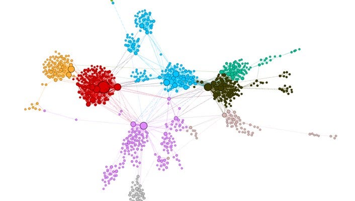
Visualizing Word Embeddings with GloVe and Word2Vec
Now, there’s a problem: word embeddings alone don’t tell the machine where a word is located in the sentence. Due to the parallel nature of it, self-attention loses the sequence of the words, which is why we require positional Encodings.
Step 2. Adding Order: Positional Encodings
Imagine reading a sentence where all the words are jumbled up. Without knowing the order, the sentence loses its meaning. To solve this, Transformers use positional encodings. These help to capture the position of the words. Let’s take another example:
“The cat, which was sitting on the mat, looked happy.”
● “cat” (position 1) → Embedding + Positional Encoding for position 1
● “mat” (position 6) → Embedding + Positional Encoding for position 6
Now, the model knows that “cat” comes before “mat.”
As to how we can do that, is continued in depth, later in the series.
Noot Noot, there’s another problem: word embeddings alone don’t tell the entire context of a word in the given sentence, it only gives the average meaning (or average context) of the word as a whole. So, to say, the embeddings only give the “static context” of the word and not the “dynamic context”.
For Example: In the sentence “River Bank Flows”, bank could have two different embeddings
● In money bank, “bank” → [0.2, 0. 7, -0.1, …]
● In river bank, “bank” → [0.5, -0.3, 0.8, …]
Which is why we require self-attention mechanism.
Step3. Brewing the magic: Self-Attention Mechanism
With words represented as numbers and their positions encoded, it’s time for the star of the show: the self-attention mechanism. As discussed earlier, the “self-attention” helps to find the relationship between each word in a sentence to the others, and captures it in the embeddings, thus forming the new vector for each word, informed by the entire context of the sentence, called the context vector.
We aim to find the relationships for any word in the sentence with all other words, by multiplying the embedding of that word with the similarity score of it with every word in the sentence individually, and then adding all of them.
In the example: “cat likes pizza.”, if the embedding of “cat” is Ec then:
● “cat” → (Ec similarity with “cat”) + (El similarity with “likes”) + (Ep *similarity with “pizza”)
Similarly, the word “likes” and “pizza” can be calculated:
Assuming embeddings as El and Ep respectively.
● “likes” → (Ec similarity with “cat”) + (El similarity with “likes”) + (Ep *similarity with “pizza”)
● “pizza” → (Ec similarity with “cat”) + (El similarity with “likes”) + (Ep *similarity with “pizza”)
We know about the embeddings already, but what is the similarity score?
Also known as the attention weights, they are simply the dot product of embeddings for the two words that we have to find similarity for. Simple as that.
So, similarity score for the words “Cat” and “Pizza” would be: (Ec).(Ep)
Finally, the vector received will be:
● “cat” → [ Ec (Ec.Ec) + El (Ec.El)+ Ep * (Ec.Ep) ]
This vector obtained is called the Context Vector.
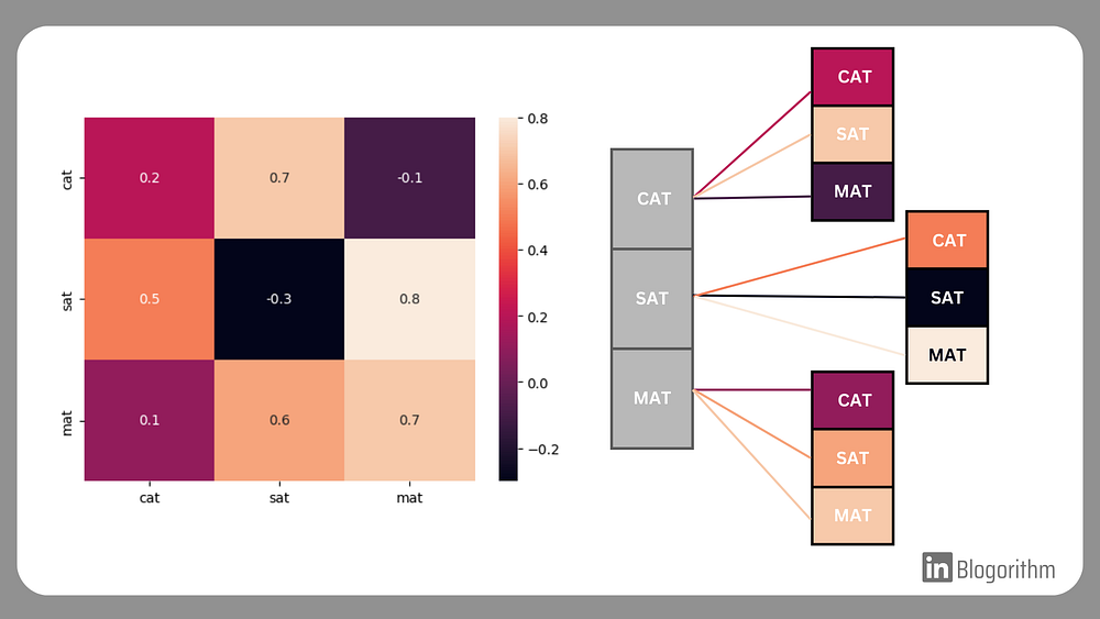
Visualizing Self-Attention Mechanism
The same process can be much better performed by using Matrices.
For a sentence of n words,
Say Matrix E is a matrix of n rows, containing the embeddings of words stacked on top of each other.
For example: In the sequence “Cat Sat Mat”,
E = [ [0.2, 0. 7, -0.1, …],
[0.5, -0.3, 0.8, …],
[0.1, 0.6, 0.7, …] ]
And Say Matrix W of order n*n = holds the similarity scores of words, also called “attention-scores”
Hence, W[i][j] = (Ei).(Ej)
In this example,
W = [ Ec.Ec Ec.El Ec.Ep ],
[ El.Ec El.El El.Ep ],
[ Ep.Ec Ep.El Ep.Ep ]
Finally, to find the context matrix Y, we use the formula:
Y= W * ET
Where ET is the transpose of matrix E.
The Y obtained is the final “token” of the words, containing the context vectors of all the words in the sequence.
Y=
[ C1 ]
[ C2 ]
[ C… ]
[ Cn ]
There are two teeny tiny details that were omitted in the previous section, giving rise to two problems. These are discussed in the next sections.
Problem 1: Queries, Keys, and Values
The Problem with the Simplified Approach is that there are no Learned Transformations. Hence, the embeddings of the words are used directly, without any learned transformations. This limits the model’s ability to capture complex relationships. Hence, we need to introduce learnable parameters in the process.
The Solution: Query, Key, and Value
Each word embedding is transformed into three vectors:
● Query (Q): Represents the word we’re focusing on.
● Key (K): Represents the word we’re comparing to.
● Value (V): Represents the information we want to extract.
These vectors are computed using learned weight matrices:
Q=E⋅WQ
K=E⋅WK
V=X⋅WV
Where WQ, WK, WV are the attention score Parameters.
For an analogy, think of it like a search engine:
● The Query is what you’re searching for.
● The Key is the index of available information.
● The Value is the actual content you retrieve.
Problem 2. SoftMax: Turning Scores into Probabilities
When the self-attention mechanism calculates attention scores (using the dot product of Queries and Keys), these scores are unbounded. This means they can take any value, making it difficult to interpret how much focus each word should receive.
For example, consider the attention scores for the word “bank” in the sentence “The bank by the river is full of money.” The scores might look like this:
● “bank” → “river”: 5.2
● “bank” → “money”: 3.8
● “bank” → “the”: 1.1
These raw scores don’t tell us how much weight to assign to each word.
The Solution: Normalization: SoftMax function
The SoftMax function converts these unbounded scores into probabilities that sum to 1. This allows the model to assign a clear, interpretable weight to each word. This process is called normalization.
How SoftMax Works:
Input: A vector of attention scores.
Output: A vector of probabilities.
Mathematically, SoftMax is defined as:
SoftMax(xi)=exi / ∑j=1 to n: exj
Where:
● xi: The attention score for the i-th word.
● n: The total number of words in the sequence.
Hence, the final form of the self-attention mechanism up untill the SoftMax function can be simply represented as: S = Softmax(Q*KT / √d_k)
Where, d_k is the Key Dimension Size.
Example:
For the attention scores [5.2, 3.8, 1.1], SoftMax might produce probabilities like:
● “river”: 0.7
● “money”: 0.2
● “the”: 0.1
Now, the model knows to focus 70% on “river”, 20% on “money”, and 10% on “the.”
The attention scores are passed through a SoftMax function, which converts them into probabilities. These probabilities determine how much focus each word should receive.
For instance, “cat” might have a high attention score with “mat” (because they’re related) and a low score with “pizza.”
Finally, we calculate the Context Vector as:
C = S . V
Where, S is the SoftMax function,
And V is the Value Vector
The context vectors of each word can be added to get the final value,
that represents the entire context of the input.
Section 5. Why Self-Attention is a Game-Changer
● Captures Long-Range Dependencies: Unlike older models, self-attention can directly model relationships between distant words.
● Parallelizable: All words are processed simultaneously, making it faster to train on modern hardware.
● Context-Aware: Each word’s representation is influenced by the entire sentence, not just its immediate neighbours.
Section 6. The Big Picture: Transformers and LLMs
The self-attention mechanism is repeated multiple times in a Transformer, with each layer refining the word representations further. By combining word embeddings, positional encodings, self-attention, and normalization, Transformers can understand and generate text with remarkable accuracy.
This technology powers modern LLMs like GPT, BERT, and T5, enabling applications like:
● Chatbots (e.g., ChatGPT)
● Machine Translation (e.g., Google Translate)
● Text Summarization (e.g., news article summaries)
The self-attention mechanism is the cornerstone of modern NLP. By enabling models to focus on the most relevant parts of a sentence, it has unlocked new levels of performance and scalability. Whether you’re building a chatbot, analysing sentiment, or translating languages, understanding self-attention is key to harnessing the power of modern LLMs.
So, the next time you interact with an AI, remember: it’s all about attention!
If you enjoyed this post, feel free to share it and follow me for more deep dives into AI and machine learning!